Effective Play Indicators (EPIs) and Overplayed Opponents – Where are the differences?
With the increasing importance of data-driven football analysis, one of the most prominently used statistics has become the number of opponents a player was able to take out of a game through a pass. It not only describes the passing quality of a player, but also gives an intuition about how offensively oriented a player is. The overplayed opponents statistic has one major issue though, it is extremely tedious to record. Every pass needs to be considered in detail, making the already lengthy process of documenting the events of the game even longer. Therefore, we at Matchmetrics were looking for a way to streamline this process. We asked ourselves: is it possible to estimate the number of overplayed opponents, simply on the basis of our passing EPI values? The short answer is a resounding yes, especially for certain player positions. Continue reading for the juicy details.
Data
To start off, we’ll need to get an overview of the data. First, we counted the number of overplayed opponents for every player from close to 2000 games. We defined an overplayed opponent as any opponent that is closer to his own goal compared to the ball before a pass, but further away after the pass. Check out the image below for a visual example. In total we obtained a dataset of 52,000+ entries.
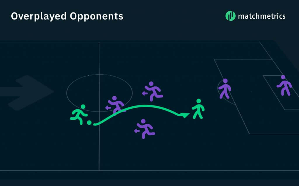
In this example the player is able to overplay 3 opponents with one pass.
By now plotting the different EPI passing values against the overplayed opponents, we can get an initial idea of how well they correlate. The EPI short passing and delivery values (left and bottom plots) show a nice relationship. The higher the EPI value becomes, the higher also the overplayed opponents value is. The long passing value (right plot) paints a different picture. Till a point of about 200 EPI passing value and 40 outplayed opponents, we can see a positive correlation (positive slope), after that point, the relationship seems to be random or even negative.
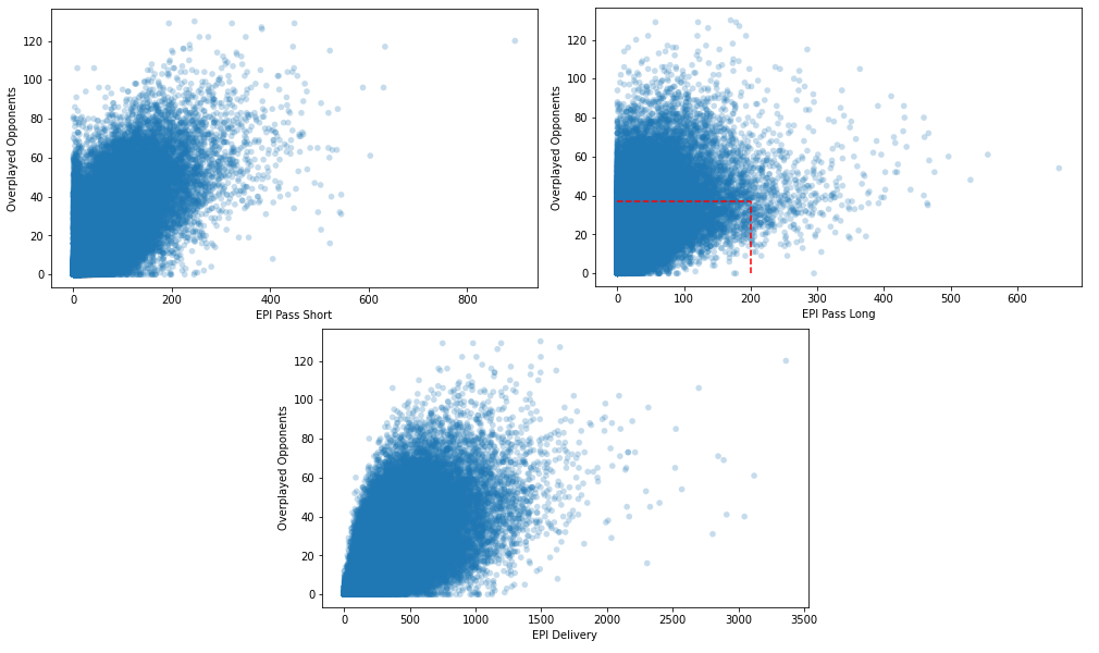
In general, the plots support the intuition quite well. The more dangerous passes a player is able to make, the more opponents he should be able to take out of the game. By computing the correlation coefficient we can check that intuition. The correlation coefficient is a value ranged between -1 and 1 that describes how strong the linear relationship between two values is. It is 0 if the relationship is completely random, -1 if we can draw a perfect line with a negative slope and +1 if we can draw a perfect line with a positive slope through all values. For the short passing value, we obtain a correlation coefficient of about 0.64, long passes correlate with the overplayed opponents with a value of circa 0.51 and delivery has a value of 0.60.
Prediction Model
Not a bad start, but we can do better. Optimally, we would like to combine the different EPI categories, as the overplayed opponents depend on all of them simultaneously. Next, we’ll throw all the EPI values into a linear model, which combines them such that they best model the overplayed opponents. Additionally, the three EPI categories don’t capture every possible pass. We’re still missing passes from free kicks or crosses, as well as goalkeeper throws etc. Let’s not go into too much detail, but we’ll include all of these into our model. The plot below is what we obtain in the end. On the x-axis, we’ve plotted the predicted overplayed opponent value, based on all the passing EPI categories. The y-axis is as always the actual overplayed opponents. At first glance, we can immediately see that the data cloud is a lot more narrow. This should mean that the correlation is higher because the relationship contains less randomness. And indeed, this is the case. We obtain a correlation value of 0.79!
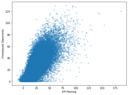
What does this value actually mean? Per se not much, other than we can predict the overplayed opponents quite well, solely on the basis of the EPI values. By calculating the absolute average difference of the prediction and the actual value, we can get an idea of how well. On average, our predictions miss the actual overplayed opponents by about 8.61. We can therefore say, on the basis of the EPI values we can estimate the number of overplayed opponents, plus-minus 8 or 9. Considering that a player can easily have up to 70 overplayed opponents in a game, that’s not too shabby.
Position Split and Seasonal Data
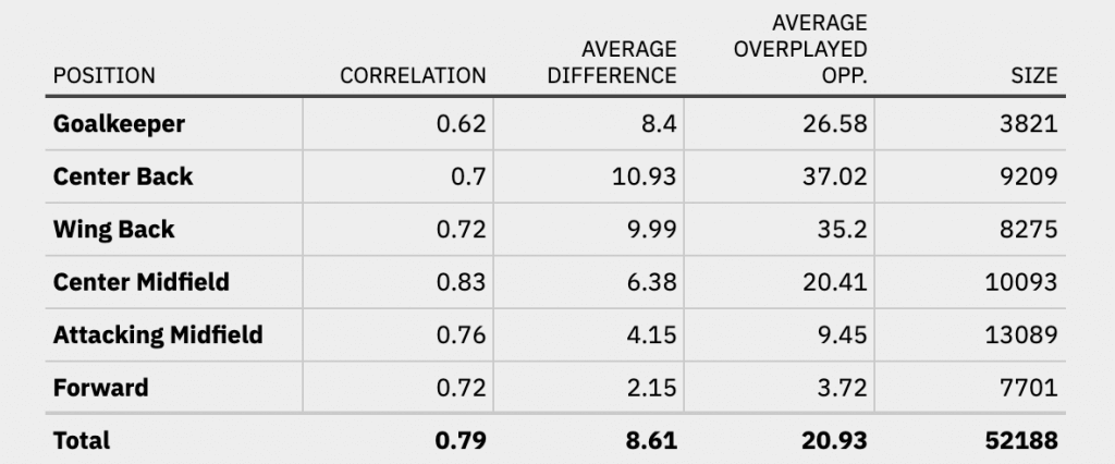
Let’s take a look at two final data augmentations: position split and seasonal data. First, it’s not a far stretch to assume that the different EPI value categories have a different degree of importance for different positions. A goalkeeper will most likely overplay more opponents through long passes into the opposing half than through short passes to his center back. Let’s first split the data by positions then and compute a linear model for each position. The table below summarizes correlation and the mean absolute difference for all positions. The rightmost columns display the average number of overplayed opponents per game and the number of data entries for that position respectively.
A couple of interesting insights can be gained from the data. First of all, the higher up the pitch a position is, the lower the number of overplayed opponents becomes. This intuitively makes sense. A forward simply has fewer players in front of him to be able to overplay. In general, the correlation is quite high for field positions, with the model being able to predict overplayed opponents the best for center midfielders. On the other hand, the correlation is lowest for goalkeepers. The reasons for this may be manifold and would require a closer investigation. Overall, the correlation is quite high though, with a value of at least 0.7 for all field positions.
Position Based Correlation
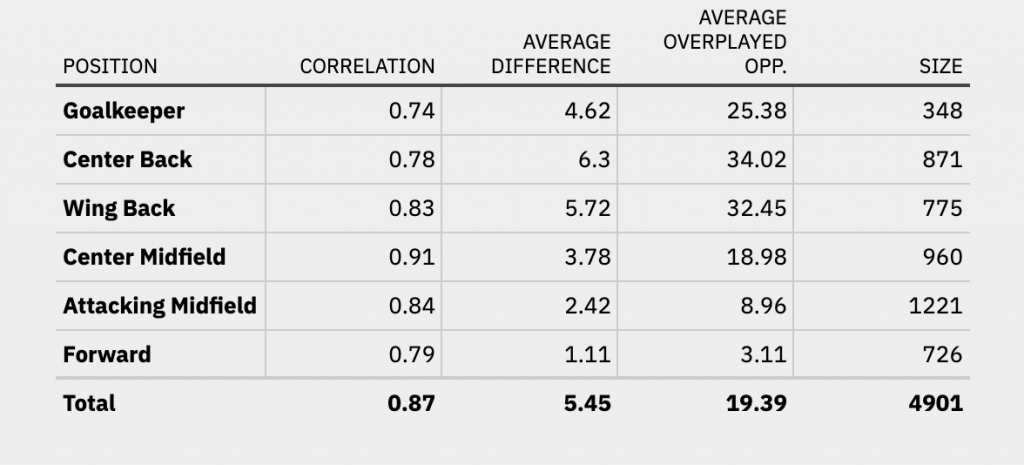
As promised, as a final step we’ll take a look at the data aggregated over an entire season. The number of overplayed opponents as well as the EPI values can vary greatly across multiple games. We can reduce that variance by taking the average values for a player across an entire season. In turn, this should improve the prediction of the model. The values for the position and season based correlation are found in the table below.
Through averaging the values across a season we can boost the correlation and almost halve the absolute average difference across the board. For every position, we can achieve a correlation of greater than 0.74 and especially for central midfielders our model can predict the overplayed opponents extremely well.
Position Based Season Correlation
So what is the takeaway from this whole analysis? In short, the tedious recording of overplayed opponents may not be necessary. By taking our EPI passing values averaged across an entire season, we can predict the number of overplayed opponents of a player to a narrow window. That being said, we might be able to squeeze out an even better prediction by switching to more expressive models.
Read more about EPIs and Scoutpanel →


